Trick 8: Keep the receipts

Numbers carry their arithmetic; claims wait for their statistics.

References. LLMs fabricate citations — fluent, plausible, non-existent, at double-digit rates for some models. Two standing instructions keep the human check cheap:

Statistics. The paper ships a ranking-statistics tutorial as an appendix, since the field has measurably gotten data analysis wrong for decades. The short form: argue with distributions, not single runs; a difference must pass two gates — significance (e.g. Kolmogorov–Smirnov) and effect size — before it earns the word “better”; ranking many treatments needs its own procedure, not pairwise p-hacking. Not every researcher is a statistician; standard AI assistance here can raise typical quality.

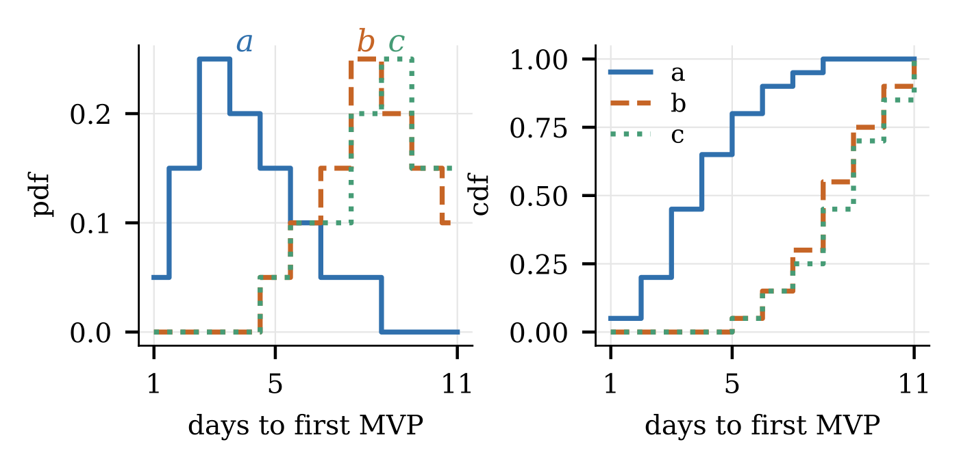
Argue with distributions, not single runs: three treatments as pdf (left) and cdf (right).

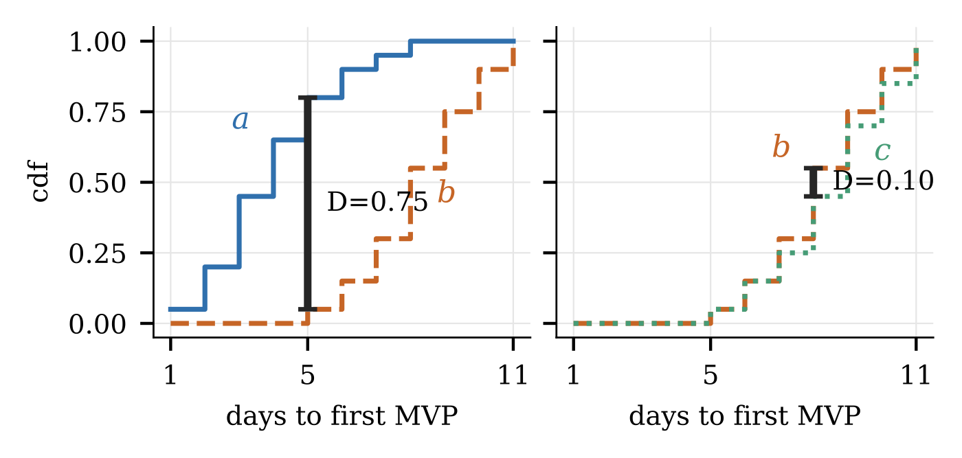
The Kolmogorov–Smirnov gate: a vs b differ (D=0.75); b vs c do not (D=0.10). Only differences that pass significance and effect size earn the word “better”.

The code

The whole kit is five functions, stdlib only, every pass linear on pre-sorted data. The gate: two treatments are the same unless significance (KS) and both effect sizes (Cliff's δ, Cohen's d) all vote different.

def same(xs, ys,
  c0=.35,   # cohen threshold (Cohen'88)
  d0=.195,  # cliffs threshold (Romano'06)
  k0=1.36,  # ks threshold (Massey'51)
  is_sorted=True):
  if not is_sorted:
    xs, ys = sorted(xs), sorted(ys)
  return (cohen(xs, ys)  <= c0 and
          cliffs(xs, ys) <= d0 and
          ks(xs, ys)     <= k0)

Significance: KS walks both sorted lists one distinct value at a time; the statistic is the largest vertical gap between the two cdfs, rescaled to critical units (under 1.36 = insignificant at the usual 5% false-alarm rate).

def ks(xs, ys):
  nx, ny = len(xs), len(ys)
  d = p = q = 0
  while p < nx and q < ny:
    v = min(xs[p], ys[q])
    while p < nx and xs[p] == v: p += 1
    while q < ny and ys[q] == v: q += 1
    d = max(d, abs(p/nx - q/ny))
  return d / ((nx+ny) / (nx*ny)) ** 0.5

Effect size, non-parametric: Cliff's δ asks how often x beats y minus how often y beats x. Naively quadratic; sorting first makes it linear.

def cliffs(xs, ys):
  gt = lt = j = k = 0
  for x in xs:
    while j < len(ys) and ys[j] < x:
      j += 1; k = j
    while k < len(ys) and ys[k] == x:
      k += 1
    gt += j; lt += len(ys) - k
  return abs(gt - lt) / (len(xs)*len(ys))

Effect size, pragmatic: Cohen's d catches differences that are real but dull — smaller than anyone cares about. No imports needed: on sorted data the 10th-to-90th percentile gap spans 2.56 standard deviations, so one subtraction estimates the deviation.

TINY = 1e-32

def mean(a):
  return sum(a) / len(a)

def stdev(a):
  n = len(a) // 10
  return (a[9*n] - a[n]) / 2.56

def cohen(xs, ys):
  n, m = len(xs), len(ys)
  sd = (((n-1)*stdev(xs)**2 +
         (m-1)*stdev(ys)**2)
        / (n+m-2)) ** 0.5
  return abs(mean(xs)-mean(ys)) / (sd+TINY)

Many treatments: no pairwise p-hacking. Sort by medians, sweep once best-to-worst; each treatment joins the current rank while same holds, else opens a new rank. Rank zero holds the winners.

def ranks(d, big=False):
  mid = lambda t: t[len(t) // 2]
  dd  = {k: sorted(v)
         for k, v in d.items()}
  out, win = {}, []
  rank, best = -1, None
  for k in sorted(dd,
                  key=lambda k: mid(dd[k]),
                  reverse=big):
    if best is None or \
       not same(dd[best], dd[k]):
      rank, best = rank + 1, k
    if rank == 0: win.append(k)
    out[k] = rank
  return win, out

Full tutorial with the worked example: the paper's Appendix B. Regenerate figures: make statsfig.

Conclusions with receipts. The conclusion retells the introduction, now with the headline numbers from the charts, each claim attached to the result that earned it. Every threat-to-validity leaf ends with a mitigation or an accepted cost — a threat without a response reads as an unfixed bug. Instrument tables (agreement rates, thresholds, download rates) live in threats, since they argue instrument validity.

And ship the package. The loop's exit condition includes a replication package — in the paper's own Reviewer-2 test run, that was the one strong point the hostile critic conceded.

Combines with: 3 — read above the knee (report the download rate); 6 — assemble critics (verifiability criterion); 4 — write to a grammar (the conclusion and threats productions enforce this).